
Executive Summary
Since 1977, Congress has instructed the Federal Reserve to promote maximum employment, stable prices, and moderate long-term interest rates. But it has mostly left the Fed to interpret what that means. How should the Fed interpret its mandate? The popular conception, which suggests there is an exploitable tradeoff between inflation and unemployment, rests on an outdated theoretical perspective I call the Naïve Phillips Curve View. The Modern Phillips Curve View, in contrast, maintains that a central bank can deliver any rate of inflation it desires, but it cannot sustain an unnatural unemployment rate. I discuss the implications of the Modern Phillips Curve View for monetary policy in theory and practice.
Key Points
The way the Fed interprets its dual mandate affects inflation, employment, interest rates, and the ability of households and businesses to plan for the future. The objectives of maximum employment, stable prices, and moderate long-term interest rates are generally complementary.
In theory, it doesn’t matter whether the Fed targets the unemployment rate at the natural rate of unemployment; the underlying (or trend) price level at the expected level consistent with low inflation; or some combination of the two.
In practice, it is difficult to determine the natural rate of unemployment and underlying price level. Consequently, the Fed’s choice of approach may affect the extent to which monetary policy achieves its objectives.
By targeting nominal spending, the Fed would better stabilize overall demand, avoid many of the practical difficulties associated with targeting unemployment or inflation directly, and more effectively achieve both sides of its mandate.
1. Introduction
In an advanced economy like the United States, money is on one side of nearly every transaction. Businesses enter contracts, make investment plans, and set prices in dollars. Workers agree to wages and are paid in dollars. Households budget, save, borrow, and spend in dollars. Their decisions in all of those transactions depend crucially on how the dollar is managed. When the dollar is managed well, the economy performs well. When the dollar is managed poorly, the economy performs poorly.
The Constitution gives Congress the power to manage the dollar. Congress, in turn, has delegated this power to the Federal Reserve, which conducts monetary policy in the United States. If the Fed’s monetary policy is too loose, prices will rise too rapidly and businesses and workers may produce more than they should. If the Fed’s monetary policy is too tight, economic activity will slow and unemployment will rise. By ensuring monetary policy is neither too loose nor too tight, the Fed helps businesses and households devise effective plans, enter appropriate contracts, and make desirable purchases.
Congress has instructed the Fed to conduct monetary policy so as to promote maximum employment, stable prices, and moderate long-term interest rates. But Congress has not fully specified how this mandate should be understood or how the Fed should act when the objectives appear to conflict. The result is a persistent source of confusion: many people believe the Fed’s mandate forces it to choose between low inflation and low unemployment. But the apparent tradeoff is largely the product of a mistaken view of monetary policy. Properly understood, stable prices and maximum employment are generally complementary goals.
In what follows, I review the Fed’s mandate and offer a sensible interpretation of the objectives. I identify the fundamental misunderstanding that leads many to conclude there is a tradeoff between the objectives of price stability and maximum employment, and I discuss the implications for monetary policy in theory and practice. Finally, I explain the dangers associated with 5Making Sense of the Federal Reserve’s Dual Mandate the Fed’s underspecified mandate and offer suggestions for more clearly specifying how the Fed should conduct monetary policy. In brief: a clearer mandate would help the Fed stabilize purchasing power, avoid unnecessary recessions, and reduce confusion about what monetary policy can and cannot do.
2. The Dual Mandate
The Federal Reserve Act requires the Fed to conduct monetary policy “so as to promote effectively the goals of maximum employment, stable prices, and moderate long-term interest rates.” Despite listing three distinct goals, this directive from Congress is commonly known as the Fed’s dual mandate: it is generally accepted — and attested in Fed documents[1] — that achieving maximum employment and stable prices “creates the conditions needed for interest rates to settle at moderate levels.”
Just as the first two objectives are generally thought to be consistent with the third, there is a sensible interpretation of “maximum employment” and “price stability” that renders the first two objectives wholly compatible, as well. In brief, the sensible interpretation defines (i) maximum employment as the rate of unemployment equal to the natural rate of unemployment and (ii) price stability as the underlying (or trend) price level that is consistent with people’s expectations and a low rate of inflation.
The natural rate of unemployment denotes the unemployment rate that prevails when no one is fooled into (a) taking a job that they would not have taken; nor, (b) not taking a job that they would have taken had they not been fooled. It is the unemployment rate that prevails when wages, prices, and expectations have had sufficient time to adjust.
Note that maximum employment does not mean zero unemployment. Even in a healthy economy, some workers are between jobs, changing industries, moving locations, or searching for a better match. The Fed can reduce unemployment caused by deficient nominal spending — that is, less total dollar spending in the economy than was anticipated. It cannot permanently eliminate unemployment that reflects ordinary labor-market frictions or deeper structural features of the economy. Put differently, monetary policy can temporarily move unemployment away from its natural rate by surprising people, but it cannot permanently keep unemployment below that rate. Hence, the sensible interpretation of maximum employment implicitly assumes that the Fed should only attempt to offset what is sometimes referred to as involuntary unemployment.
The underlying price level denotes the level of prices that would prevail after any effects of temporary supply shocks have been removed. Hence, the sensible interpretation of price stability implicitly acknowledges that the Fed should not attempt to offset temporary deviations in the price level that result from supply shocks. Sometimes such a policy is described as “looking through supply shocks.”[2]
The low rate of inflation referenced in the sensible interpretation of price stability is admittedly ambiguous. As Luther (2020) explains, economists disagree to some extent about the optimal rate of inflation over the longer run.[3] Most of the academic papers surveyed by Diercks (2019)[4] — and the most highly-cited papers, at that — generally recommend a properly measured inflation rate around 0 percent, which would tend to minimize unnecessary price adjustments.[5] Many papers find that a slightly negative rate of inflation is desirable, which is consistent with the Friedman (1969) rule.[6] Some papers, most of which were published after the 2008 financial crisis, find that a slightly positive rate of inflation is ideal, either because it lubricates labor markets [7] or reduces the odds of reaching the effective lower bound.[8] The Fed currently aims to deliver 2 percent inflation per year, as measured by the Personal Consumption Expenditures Price Index (PCEPI). For the purposes of this paper, one might remain agnostic about the optimal rate of inflation or substitute in his or her view of the ideal, be it 2 percent or otherwise. It is sufficient to accept that some low rate is ideal, regardless of whether that low rate is thought to be zero, slightly negative, or slightly positive.[9]
The sensible interpretation of the dual mandate follows naturally from the sensible interpretations of “maximum employment” and “price stability” 7Making Sense of the Federal Reserve’s Dual Mandate discussed above. In this view, the Fed should conduct policy to help ensure the unemployment rate coincides with the natural rate of unemployment and the underlying price level is consistent with people’s expectations and a low rate of inflation. As discussed below, this interpretation of the dual mandate is consistent with standard macroeconomic theory, which means it does not saddle the Fed with an obligation to do what cannot be done. However, the sensible interpretation advanced herein is out of sync with the popular conception of the dual mandate.
3. Popular (Mis-)Conception
In popular discourse and journalistic accounts, it is common to describe members of the Federal Open Market Committee (FOMC) as “hawks” or “doves,” where hawks want low inflation and doves want a low unemployment rate. More generally, one might think of a continuum from pure hawk to pure dove, with a particular FOMC member’s position determined by the relative weight he or she places on each objective. Hence, an FOMC member who places more weight on the inflation component of the dual mandate is described as hawkish whereas a member placing more weight on the employment component is described as dovish. Moreover, the relative weight placed on the inflation and employment components is generally thought to reflect the FOMC members’ preferences for inflation and employment.
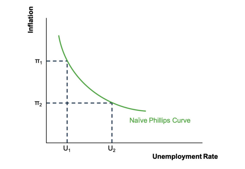
The usual hawk-dove distinction only makes sense in the context of what I will call the Naïve Phillips Curve View. This view, originally expressed by Paul Samuelson and Robert Solow (1960) [10], who drew on the earlier work of A. W. Phillips (1958) [11], treats inflation and unemployment as a menu of policy options.[12] Consider the naïve Phillips curve, depicted in Figure 1, below. The central bank can choose any point along the curve. For example, it might enjoy a lower rate of inflation if it is willing to put up with a higher rate of unemployment; or, it might enjoy a lower rate of unemployment if it is willing to put up with a higher rate of inflation. Given the supposed tradeoff between inflation and unemployment in the Naïve Phillips Curve View, it makes sense to wonder whether (and to what extent) an FOMC member prefers low inflation or low unemployment.
Figure 1. The Naïve Phillips Curve View
Many economists came to accept the Naïve Phillips Curve View in the 1960s. It is not difficult to understand why they did so. The available data, presented in Figure 2-A, next page, revealed a negative relationship between inflation (as measured by PCEPI) and the unemployment rate. And two of the most prominent members of the economics profession were claiming this negative relationship could be exploited. “During the 1960s,” Snowden and Vane (2006, p. 140) [13] write, “the Phillips (1958) curve was quickly taken on board as an integral part of the then-dominant orthodox Keynesian paradigm, not least because it was interpreted by many orthodox Keynesians as implying a stable long-run tradeoff which provided the authorities a menu of possible inflation-unemployment combinations for policy choice.”
Figure 2-A. Inflation and Unemployment, 1960s
Source: Bureau of Labor Statistics; Bureau of Economic Analysis. Inflation measured as the percent change from a year ago in the PCEPI.
Cracks in the consensus soon developed, however. In a presidential address delivered to the American Economic Association in December 1967 and published a few months later, Milton Friedman (1968, p. 11)[14] cautioned against efforts to exploit the supposed Phillips curve relationship:
[…] there is always a temporary trade-off between inflation and unemployment; there is no permanent trade-off. The temporary trade-off comes not from inflation per se, but from unanticipated inflation, which generally means, from a rising rate of inflation. The widespread belief that there is a permanent trade-off is a sophisticated version of the confusion between “high” and “rising” that we all recognize in simpler forms. A rising rate of inflation may reduce unemployment, a high rate will not.
As Friedman (1960, p. 11) explained, the monetary authority can determine the rate of inflation or other nominal quantities. But it “cannot use its control over nominal quantities to peg a real quantity — the real rate of interest, the rate of unemployment, the level of real national income, the real quantity of money, the rate of growth of real national income, or the rate of growth of the real quantity of money.”
Edmund Phelps (1967, 1968) offered a similar view around the same time.[15] Like Friedman, Phelps explained that unemployment would tend toward the economy’s natural rate, which is consistent with people’s preferences given the available technology and constraints. Phelps and Friedman acknowledged that expansionary monetary policy might temporarily fool people into working more than they otherwise would. Specifically, if workers observe higher nominal wage offers but are slow to recognize the corresponding increase in prices, they will mistakenly believe their real (i.e., inflationad-justed) wages have risen and may choose to work more. To the extent that this effect works on the extensive margin as well, the prevailing unemployment rate will temporarily fall below its natural rate as the price level rises above the level that was expected. The economic statistician will record a rise in inflation and a decline in the unemployment rate, just as adherents of the Naïve Phillips Curve View would expect.
The difference between Samuelson and Solow, on the one hand, and Friedman and Phelps, on the other, concerns what happens next. For Samuelson and Solow, the long run is “merely the consequence of a series of Keynesian short runs,” with no automatic adjustment mechanism to ensure the unemployment rate ultimately returns to the natural rate.[16] This view implicitly assumes that workers can be consistently and persistently fooled into working more than they would like given the actual real wages on offer. For Friedman and Phelps, in contrast, those workers will eventually wise up: they will come to realize that the dollars they have received in exchange for their labor services buy fewer goods and services than they had anticipated. And, as those workers who learn that their real wage is less than the real wage they are willing to accept exit employment to search for higher-paying jobs or enjoy their leisure time, the unemployment rate returns to the natural rate.
Contractionary monetary policy works in the opposite direction. If workers observe lower nominal wage offers but are slow to recognize the corresponding decrease in prices, they will mistakenly believe their real wages have fallen and may choose to exit employment in order to search for higher-paying jobs or enjoy more leisure. Correspondingly, the prevailing unemployment rate will temporarily rise above the natural rate of unemployment as the price level falls below the level that was expected. But here too, the perceived negative relationship between inflation and the unemployment rate will not last. Eventually, workers will recognize the change in prices and return to jobs offering a sufficiently high real wage. As they do, the unemployment rate will return to the natural rate.
By developing the natural rate hypothesis and explaining the important role of expectations, Friedman and Phelps offered an alternative to the Keynesian consensus. They acknowledged that one might observe a negative relationship between inflation and the unemployment rate in the short run, while explaining why that relationship will break down in the long run if the central bank attempts to exploit it. Since the natural rate of unemployment reflects the decisions people make when they are not fooled, and since people will not remain fooled forever, the Phillips curve will ultimately adjust to ensure that the rate of unemployment prevailing in the economy is consistent with the natural rate of unemployment.
If the theoretical work of Friedman and Phelps introduced a crack in the Keynesian consensus, empirical developments in the 1970s would see that consensus crumble. Inflation, which averaged 4.9 percent over the twelve months ending January 1970, climbed to 11.1 percent by January 1975. But, contrary to the Naïve Phillips Curve View, the rise in inflation did not bring about a fall in the unemployment rate: the unemployment rate rose from 3.9 percent in January 1970 to 8.1 percent in January 1975. This stagflation — a concurrence of high inflation and high unemployment — appeared to validate Friedman and Phelps.
Figure 2-B. Inflation and Unemployment, 1960s–2020s
Source: Bureau of Labor Statistics; Bureau of Economic Analysis. Inflation measured as the percent change from a year ago in the PCEPI.
Any remaining faith in the Naïve Phillips Curve View should have been eliminated by the subsequent data, presented in Figure 2-B, above, which confirms the lack of a stable, long-run tradeoff between inflation and the unemployment rate. The unemployment rate rose from 6.3 percent in January 1980 to 10.8 percent in November 1982, while inflation declined from 10.5 percent to 5.0 percent. Then, as inflation declined further to 1.6 percent in January 1987, the unemployment rate fell to 6.6 percent. Contrary to the Naïve Phillips Curve View, but consistent with the alternative offered by Friedman and Phelps, inflation and unemployment moved in the same direction over this latter period. The relationship was negative in the early 1990s, before turning positive again. It remained positive over the first half of the 2010s, before turning negative again.
Even when the relationship is generally negative for an extended period, it is not typically stable. The Phillips curve, if it exists at all, appears to have experienced at least two distinct shifts in the 2000s. Likewise, three distinct negative slopes can be estimated for the periods January 2020 to October 2020, November 2020 to June 2022, and July 2022 to present. There is, in other words, no stable tradeoff between inflation and the unemployment rate.
Greg Mankiw and Ricardo Reis (2018, p. 82) describe “Friedman’s 1967 AEA presidential address as marking a turning point in the history of macroeconomic research.” It marked the end — or, at least the beginning of the end — of the Naïve Phillips Curve View. Subsequent work by Robert Lucas and Leonard Rapping (1969)[17], Lucas (1972)[18], Finn Kydland and Edward Prescott (1977)[19], Robert Barro and David Gordon (1983a,b)[20], and others stressed the importance of expectations and advanced the natural rate hypothesis. In their Modern Phillips Curve View, there is a negative relationship between inflation and the unemployment rate, but it is not a stable, long-run relationship that a central bank might exploit. As in Friedman and Phelps, the position of the Phillips curve depends on expectations: people might be temporarily fooled into working or not working, but only to the extent that they are surprised. Even then, people will soon come to realize their mistakes, adjust their expectations, and revise their employment decisions accordingly. In the long run, the unemployment rate will coincide with the natural rate.
The Modern Phillips Curve View would later be embedded in now-standard New Keynesian models. For example, Richard Clarida, Jordi Gali, and Mark Gertler (1999)[21] write the New Keynesian Phillips curve by describing inflation at some point in time as a function of the output gap — that is, the deviation of economic output from its natural rate — and the expectation of future inflation.[22] Note that, as in the earlier works discussed above, a change in expected inflation causes the New Keynesian Phillips curve to shift, ensuring that unemployment is equal to the natural rate of unemployment when expected inflation is equal to actual inflation. And, although the New Keynesian Phillips curve is typically expressed in terms of an output gap rather than an unemployment gap, both gaps denote a deviation in a real variable relative to its natural rate. Hence, standard New Keynesian models, which now dominate the macroeconomics profession and are widely-used at central banks around the world, fully embrace the natural rate hypothesis and recognize the importance of expectations.
4. Optimal Monetary Policy in Theory
The key takeaway from the Modern Phillips Curve View is that a central bank can deliver any rate of inflation it desires, but it cannot sustain an unnatural rate of unemployment. If it tries to push the unemployment rate below its natural rate, by delivering a higher rate of inflation than people expect, inflation expectations will rise. If it tries to hold the unemployment rate above its natural rate, by delivering a lower rate of inflation than people expect, inflation expectations will fall. In both cases, the deviation of the unemployment rate from the natural rate will be eliminated as expectations adjust and people revise their employment decisions in light of their preferences, constraints, and available technology.
In theory, it does not matter whether the Fed:
Targets the unemployment rate at the natural rate of unemployment;
Targets the underlying price level at the expected level consistent with low inflation; or
Adopts a combined approach whereby it (explicitly or implicitly) puts some weight on each of the two targets identified above.
To understand why this is, recall that the unemployment rate deviates from the natural rate when people are fooled into working or not working. If the Fed conducts monetary policy such that the unemployment rate is equal to the natural rate of unemployment, it follows that no one has been fooled — i.e., that the underlying price level is at the expected level, which is consistent with low inflation. Alternatively, if the Fed announces a credible inflation target and then conducts monetary policy such that the underlying price level is at the expected level at each future point in time, it follows that no one will be fooled by unexpected inflation — and, hence, that the unemployment rate will be equal to the natural rate of unemployment. Finally, since the first two strategies amount to describing the same monetary policy in two distinct but equivalent ways, it will yield the same results as a weighted average of the two approaches. Economists call this the divine coincidence, since achieving one of the objectives implies that the other objective will be achieved as well — a meaningful alignment of circumstances that feels too purposeful to be mere random chance.[23]
Figure 3. The Modern Phillips Curve View
To understand the divine coincidence, consider the simple graphical model presented in Figure 3, above. Inflation is measured on the vertical axis. The unemployment rate is measured on the horizontal axis. Suppose the central bank is given a dual mandate, whereby it seeks to deliver some given rate of inflation, π , while ensuring that the unemployment rate is equal to the natural rate of unemployment, U. Suppose further that the public is aware of the mandate and believes the central bank is credibly committed to delivering on its stated objectives. In that case, the public will set their inflation expectations in line with the central bank’s stated objectives. Correspondingly, the Phillips curve conditional on those expectations will intersect a vertical line at that natural rate of unemployment. So long as inflation is equal to the expected rate of inflation, the unemployment rate will equal the natural rate of unemployment.
The stable equilibrium in Figure 3, previous page, is at the unique point where inflation is equal to the central bank’s desired rate of inflation and the unemployment rate is equal to the natural rate of unemployment. To achieve this unique equilibrium, the central bank can conduct monetary policy such that the unemployment rate is equal to the natural rate of unemployment, in which case the Phillips curve will ensure inflation is equal to the central bank’s desired rate of inflation. Alternatively, the central bank can conduct monetary policy such that inflation is equal to the central bank’s desired rate of inflation, in which case the Phillips curve will ensure the unemployment rate is equal to the natural rate of unemployment. Conditional on expectations (and, hence, the position of the Phillips curve), either strategy — or any combination of the two — will result in the same monetary policy and, hence, the same outcome. If the central bank targets any inflation rate other than its desired rate of inflation or any unemployment rate other than the natural rate of unemployment, inflation will deviate from the central bank’s desired rate of inflation and the unemployment rate will deviate from the natural rate of unemployment until expectations adjust and the Phillips curve shifts to ensure the unemployment rate is equal to the natural rate of unemployment. But there is no systematic trade-off between inflation and unemployment. The two objectives are complementary.
For ordinary households and businesses, the implication is straightforward: the Fed best supports employment not by trying to force unemployment below its sustainable level, but by allowing the unemployment rate to reflect the well-informed plans of households and businesses. In theory, the Fed can do this by targeting the natural rate of unemployment, targeting inflation, or adopting a combined approach. In each of these cases, the Fed prevents unnecessary swings in nominal (or total dollar) spending in the economy and, in doing so, helps households and businesses make appropriate decisions in the labor market.
5. Stakeholder Statutes of the 1980s
The divine coincidence of inflation and employment objectives implies the Fed will achieve both objectives by achieving either. But practical difficulties associated with achieving the objectives may result in very different outcomes depending on which approach the Fed takes.
Suppose, for example, the Fed conducts monetary policy by targeting the unemployment rate at the natural rate of unemployment. This approach is easier said in theory than done in practice. The Fed cannot observe the natural rate of unemployment. Moreover, since technology grows in fits and starts, there is no reason to think the natural rate of unemployment is stable over time. Targeting the unemployment rate, therefore, amounts to aiming at an invisible, moving target. If the Fed could ensure the unemployment rate is always equal to the natural rate, it would generally ensure, by divine coincidence, that the underlying price level is at the expected level as well. But the Fed cannot reliably ensure the unemployment rate is equal to the natural rate because it does not know (with a reasonable degree of precision) what the natural rate of unemployment is at any point in time.
Suppose, instead, the Fed conducts monetary policy by targeting the underlying price level at the expected level consistent with low inflation. The desired rate of inflation — and, hence, the desired price level — is observable as a long-run objective. But, in the short run, temporary changes in productivity growth and other supply-side factors may cause the price level to diverge from the underlying price level. The Fed does not observe the underlying price level.[24] Hence, it knows which direction the price level should go in the long run. But it does not know (with a reasonable degree of precision) the extent to which the underlying price level deviates from the expected level nor how long it should permit the observed price level to remain above or below its long-run target.
The conventional approach, today, is to conduct monetary policy by adjusting a policy rate with guidance from a Taylor-type rule that places some weight on each of the two objectives.[25] The Fed incorporates various Taylor-type rules in its macroeconomic models and also reports the guidance prescribed by five such rules in its semiannual Monetary Policy Report.[26] Although the Fed is not bound by any of these rules, they nonetheless inform the FOMC’s rate-setting decisions.
Consider, for example, a monetary policy rule for the policy rate where the Fed’s nominal interest rate target recommended at a given time is equal to the neutral rate — that is, the rate consistent with productivity growth, population growth, people’s preferences for current relative to future consumption, and the Fed’s desired inflation rate — plus an adjustment term. The adjustment term recommends increasing (decreasing) the nominal interest rate target when there is a positive (negative) inflation gap — that is, the difference between inflation and the Fed’s inflation target. It recommends decreasing (increasing) the nominal interest rate target when there is a positive (negative) unemployment gap — that is, the difference between the unemployment rate and the natural rate of unemployment. The magnitude of the adjustment depends on the magnitudes of the inflation and output gaps and the weight placed on each term. If both the inflation gap and unemployment gap are positive (negative), the direction of adjustment depends on the weight placed on each term.
Economists debate how much weight the Fed should place on the inflation gap relative to unemployment or output gaps.[27] But this debate, which is often misconstrued in popular discourse and journalistic accounts, must be understood in light of the divine coincidence and practical considerations discussed above. Those economists who recommend placing more weight on the inflation gap are not typically “hawks” in the sense that they care more about inflation than unemployment. Rather, they advise placing more weight on the inflation gap because they believe doing so will enable the Fed to more effectively achieve both objectives. Remember: the objectives are complementary. If the Fed achieves one, it will also achieve the other. The relevant question, therefore, is not about the desirability of lower inflation or lower unemployment. Rather, it concerns the practical difficulties of targeting inflation and unemployment.
Rather than targeting an average of inflation and unemployment gaps, the Fed might target the nominal spending gap — i.e., the difference between actual and desired nominal gross domestic product (GDP).[28] Targeting a nominal spending gap has several advantages.[29]
First, it permits the Fed to achieve its desired inflation in the long run by setting its desired nominal spending growth equal to the sum of the average — or, trend — rate of real GDP growth and the Fed’s desired inflation rate.
Second, since nominal spending is the product of real GDP and the price level, successfully targeting the nominal spending gap necessarily implies a countercyclical price level: adverse supply shocks cause the price level to rise above the underlying price level, whereas favorable supply shocks cause the price level to fall below the underlying price level.
Third, since the price level only deviates from the underlying price level to the extent that is warranted by temporary supply conditions, there is no need to discern the extent to which changes in the price level are warranted — and, correspondingly, whether a change in the price level reflects a change in the underlying price level.
Fourth, since the underlying price level is stable when the Fed targets the nominal spending gap, the unemployment rate will coincide with the natural rate of unemployment.
Taken together, targeting the nominal spending gap enables the Fed to hit its desired long-run inflation target, allows prices to reflect genuine changes in relative scarcity in the short run, alleviates the need to determine whether changes in the price level are driven by supply or demand shocks, and keeps the economy at or near full employment. These advantages imply the Fed will more effectively achieve its inflation and employment objectives by targeting the nominal spending gap.
6. Dual Mandate Danger
Thus far, I have adopted a sensible interpretation of “maximum employment” and “price stability” and explained how the Fed might achieve both objectives. One risk in giving the Fed its dual mandate, however, is that it will not adopt such a sensible interpretation or will not account sufficiently for the practical difficulties considered above. Consequently, it may respond too slowly to inflation, too aggressively to supply shocks, or in ways that promise more employment than monetary policy can sustainably deliver. Two examples serve to illustrate.[30]
6.1 The Post-pandemic Inflation
In August 2020, the Fed revised its Statement on Longer-Run Goals and Monetary Policy Strategy — henceforth, the consensus statement.[31] The changes made to the consensus statement in 2020 strongly suggest that the Fed was redirecting attention from price stability to maximum employment.[32] The changes — along with statements from Fed officials — also suggest that the Fed had reinterpreted its maximum employment mandate to address issues of inequality, which is not generally consistent with the standard natural rate view outlined above. These changes may partly explain why the Fed was so slow to combat above-target inflation in 2021 and early 2022.
What changes did the Fed make to its consensus statement? Whereas the Fed had previously written that it would conduct monetary policy to mitigate “deviations of employment from the Committee’s assessments of its maximum level,” it indicated in the revised consensus statement that it would aim to “mitigate shortfalls of employment from the Committee’s assessments of its maximum level.” As Peter Ireland (2025, p. 1257) has noted, this change strongly suggests the Fed moved “away from the natural rate hypothesis and towards Samuelson and Solow’s view of a (now more favorable) trade-off of higher inflation in exchange for lower unemployment.”[33] Ireland also highlights the Fed’s description of “maximum employment but not inflation as a ‘broad based and inclusive goal’” and its replacement of the so-called balanced approach with an asymmetric approach that considers employment shortfalls and inflation deviations.[34] In other words, the Fed would err toward running the economy hot, preferring a lower unemployment rate despite the risk of higher inflation.
Why did the Fed feel compelled to state that maximum employment was a broad-based and inclusive goal? Why did it not feel compelled to state that price stability was a broad-based and inclusive goal?
Louis Rouanet and Alexander William Salter (2024) argue that the Fed began viewing the reduction of inequality as part of its mission and, consistent with this mission creep, began “focusing on racial unemployment gaps.”[35] They review speeches by Fed officials and find “a recent and growing interest” in social justice topics, which they describe as “particularly acute concerning diversity and racial topics.” They suggest the “revival of Phillips-curve thinking at the Fed” is at least in part due “to more expansive employment goals.”
If the Fed’s revised language was intended to create space to address racial unemployment disparities, that’s a worrisome development. Given the structural features of the economy that generate unequal outcomes in employment, reducing inequality would generally require the Fed to “improve upon” the natural rate of unemployment. However, as discussed above, such efforts have at most a temporary effect on unemployment (and, hence, the differences in unemployment rates across races) and a permanent effect on the level of prices.
The alleged shift in views may explain the Fed’s slow response to rising inflation in 2021 and early 2022. Bryan Custinger and I have shown that the FOMC did not publicly acknowledge inflation was at least partly due to an increase in nominal spending until December 2021, though that should have been clear by September 2021.[36] Even then, they did not adjust their policy rate until March 2022 — and did not achieve a positive real (i.e., inflation-adjusted) federal funds rate until July 2022. It is difficult to argue that the FOMC would have waited so long to tighten monetary policy had it been focusing exclusively on price stability.
6.2 Tariff Concerns
In 2025, Fed officials expressed concerns that President Trump’s tariff policies might prevent them from delivering both price stability and maximum employment — i.e., that they might need to choose between the two. Statements from Fed officials suggested widespread agreement that the Fed should look through any price effects of a tariff, so long as such effects did not cause inflation expectations to rise. However, those statements also suggested Fed officials were inclined to interpret any upward movement in the unemployment rate as an indication that they were performing worse on the employment portion of their mandate. In other words, Fed officials were either ignoring potential changes in the natural rate of unemployment or interpreting the employment mandate as something other than ensuring the unemployment rate coincided with the natural rate of unemployment.
To see how Fed officials expected higher tariff rates to affect inflation and unemployment, consider the change in the median FOMC member’s projections from December 2024 to June 2025. In December 2024, the median FOMC member projected 2.5 percent inflation — as measured by PCEPI — and a 4.3 percent unemployment rate for 2025.[37] In June 2025, the median FOMC member projected 3.0 percent inflation and a 4.5 percent unemployment rate for 2025.[38] Hence, Fed officials increased their projections for inflation and the unemployment rate as they learned that tariffs would be higher than previously expected.
To the extent that higher tariff rates cause prices to rise, they do so by constraining supply, not by boosting demand. As noted above, the Fed should generally look through supply-driven changes in the price level.[39] There is some risk, however, that an adverse supply shock will cause people to expect persistently higher inflation. In that case, the Fed should take a second-best approach: restricting (or maintaining a restrictive) policy to anchor expectations on the Fed’s preferred inflation rate.
To the extent that higher tariff rates constrain supply, they may also cause the natural rate of unemployment to rise. Again: the Fed should not generally respond to supply shocks. Higher unemployment may be an unwelcome side effect of higher tariff rates, but the Fed cannot maintain an unemployment rate below the natural rate of unemployment — and trying to do so will result in even higher prices than is necessary given the higher tariff rates.
Alas, Fed officials did not seem to see it that way. In a talk at the Economic Club of New York in June 2025, then-Governor Adriana Kugler noted “the prospect that trade and other policy changes could raise the unemployment rate and push employment away from our objective.”[40] Governor Lisa Cook expressed similar concerns in a talk at the Council on Foreign Relations. “Trade policy changes and the response of financial markets, firms, and consumers suggest risks to both sides of our dual mandate,” she said.
In September 2025, then-Fed Chair Jerome Powell described “a challenging situation,” where near-term “risks to inflation are tilted to the upside and risks to employment to the downside.”[41] Vice Chair Philip Jefferson similarly noted “that both sides of our mandate are under pressure.”[42]
If Fed officials held the sensible interpretation of maximum employment described above, they would not describe a tariff-induced rise in the unemployment rate as pushing employment away from their objective. Likewise, they would not describe the prospect of a tariff-induced rise in the unemployment rate as a risk to the maximum employment portion of their mandate. Rather, they would state that, to the extent higher tariffs cause unemployment to rise, it does so by increasing the natural rate of unemployment. Instead, they appeared to ignore potential changes in the natural rate of unemployment or interpret the employment mandate as something other than targeting the unemployment rate at the natural rate of unemployment. Either way, the effect was to encourage looser monetary policy — and higher inflation — than was justified by the tariffs.
7. Policy Recommendations
Congress might eliminate the popular (but mistaken) conception that it has asked the Fed to achieve two incompatible objectives without compromising the Fed’s ability to promote maximum employment and stable prices. It can do this by replacing the current, poorly-defined dual mandate with a single mandate designed to achieve both objectives.
The clearest way to do that would be to specify a nominal spending target anchored to a low rate of inflation. The next-best alternative would be to specify a symmetric average inflation target.[43] Although a single mandate aimed at ensuring the unemployment rate coincides with the natural rate of unemployment works in theory, the comparative difficulty of estimating the natural rate of unemployment makes an unemployment target undesirable in practice. As discussed above, the lack of an explicit employment objective would not imply employment is unimportant or less important than inflation. It would merely be to acknowledge that the Fed can more effectively promote maximum employment by targeting nominal spending or the average rate of inflation.
If Congress is unable or unwilling to specify a single mandate for the Fed, it might instead take the comparatively smaller step of clarifying how the Fed should interpret its dual mandate. Ideally, Congress would indicate that, by maximum employment, it means the rate of unemployment that is consistent with the natural rate of unemployment and, by stable prices, it means an underlying (or, trend) price level that is consistent with expectations and a low rate of inflation. By more clearly specifying what the Fed should do, Congress would enable the Fed to focus more narrowly on how to go about doing it.
A clearer mandate would help the Fed stabilize purchasing power, avoid unnecessary recessions, and reduce confusion about what monetary policy can and cannot do. The goal is not to make the Fed care less about employment or more about price stability. Rather, it is to give the Fed a mandate that will enable it to more effectively achieve its employment and price stability objectives. When properly understood, stable prices and maximum employment are not rival goals. They only become rival goals when the Fed attempts — or, is instructed by Congress — to deliver more employment than monetary policy can sustainably deliver. If, instead, it aims to stabilize nominal spending, it will simultaneously promote maximum employment and stable prices.
8. Conclusion
Congress has instructed the Fed “to promote effectively the goals of maximum employment, stable prices, and moderate long-term interest rates.” But it has mostly left the Fed to interpret what that means. I have offered a sensible interpretation based on now-standard macroeconomic theory: maximum employment means employment consistent with the natural rate of unemployment and stable prices means an underlying — or trend — price level consistent with expectations and a low rate of inflation.
The Fed does not generally face a tradeoff between its maximum employment and price stability objectives when those objectives are sensibly defined. Whereas the Naïve Phillips Curve View treats inflation and unemployment as a menu of policy options, the Modern Phillips Curve View recognizes the limits of monetary policy: the Fed can deliver a low and predictable rate of inflation over time, but it cannot permanently sustain an unemployment rate below the natural rate.
In theory, the Fed can achieve both sides of its mandate by targeting the unemployment rate at the natural rate, the underlying price level at the expected level consistent with low inflation, or some combination of the two. In practice, however, the natural rate of unemployment and the underlying price level are difficult to observe. As a result, the Fed’s choice of operating framework matters. A nominal spending target would avoid many of these practical difficulties by stabilizing total dollar spending while allowing prices and employment to adjust to real changes in supply conditions. Actual Fed policy appears to deviate from this approach. In recent years, Fed officials have sometimes ignored potential changes in the natural rate of unemployment or interpreted the employment mandate as something other than targeting the unemployment rate at the natural rate of unemployment. That risks making the dual mandate appear more conflicted than it really is and may also result in higher inflation. The central lesson is that monetary policy can best promote both stable prices and maximum employment when the Fed’s objectives are defined in terms of what monetary policy can sustainably achieve.
End Notes
[1] Federal Reserve Board. “Monetary Policy: What Are Its Goals? How Does It Work?” Note, July 29, 2021.
[2] For example, in a Federal Reserve Staff Paper prepared for the 2025 framework review, Hess Chung and coauthors acknowledge “optimal monetary policy allows inflation to depart from the target in response to certain supply shocks or in cases when sectoral dynamics are relevant,” so long as “inflation expectations remain well anchored.” Chung, Hess, Callum Jones, Antoine Lepetit, and Fernando M. Martin (2025). Implications of Inflation Dynamics for Monetary Policy Strategies. Finance and Economics Discussion Series (2025-072).
[3] Luther, William J. “Four principles for a base money regime.” Cato Journal, 40 (2020): 533.
[4] Diercks, Anthony M. (2019) “The Reader’s Guide to Optimal Monetary Policy.” Available at http://dx.doi.org/10.2139/ssrn.2989237.
[5] Mankiw, N. Gregory. (1985) “Small Menu Costs and Large Business Cycles: A Macroeconomic Model of Monopoly.” Quarterly Journal of Economics 100 (2): 529–37.
[6] Friedman, Milton, 1969, The optimum quantity of money, in: M. Friedman, ed., The Optimum Quantity of Money and Other Essays (Aldine, Chicago, 1L).
[7] See, for example: Akerlof, George, William Dickens, and George Perry. “Low inflation or no inflation: Should the Federal Reserve pursue complete price stability?” Challenge 39.5 (1996): 11-17.
[8] See, for example: Coibion, Olivier, Yuriy Gorodnichenko, and Johannes Wieland. “The optimal inflation rate in New Keynesian models: should central banks raise their inflation targets in light of the zero lower bound?” Review of Economic Studies 79.4 (2012): 1371-1406.
[9] On the optimal rate of inflation, see: White, Lawrence H. “Should the Federal Reserve raise its inflation target?.” Southern Economic Journal 91.4 (2025): 1372-1390.
[10] Samuelson, Paul A., and Robert M. Solow. “Analytical aspects of anti-inflation policy.” The American Economic Review 50.2 (1960): 177-194.=59.
[11] Phillips, Alban W. “The relation between unemployment and the rate of change of money wage rates in the United Kingdom, 1861-1957.” Economica 25.100 (1958): 283-299.
[12] To their credit, Samuelson and Solow (1960, p. 193) cautioned the reader against assuming the menu is fixed: “All of our discussion has been phrased in short-run terms, dealing with what might happen in the next few years. It would be wrong, though, to think that our Figure 2 menu that relates obtainable price and unemployment behavior will maintain its same shape in the longer run. What we do in a policy way during the next few years might cause it to shift in a definite way.” But that caution appears to have been largely ignored. As Mankiw and Reis (2018) note, “these effects were considered caveats to their main analysis, rather than central to it. For most readers of their paper, the main take-away was the Phillips curve as a menu of outcomes available to policymakers, both in the short run and in the long run.” Mankiw, N. Gregory, and Ricardo Reis. “Friedman’s presidential address in the evolution of macroeconomic thought.” Journal of Economic Perspectives 32.1 (2018): 81-96.
[13] Snowden, Brian and Howard R. Vane, 2006. Modern Macroeconomics: Its Origins, Development, and Current State. Cheltenham: Edward Elgar.
[14] Friedman, Milton. “The Role of Monetary Policy.” American Economic Review 58, no. 1 (1968): 1-17;
[15] Phelps, Edmund S. “Phillips curves, expectations of inflation and optimal unemployment over time.” Economica (1967): 254-281; Phelps, Edmund S. “Money-wage dynamics and labormarket equilibrium.” Journal of Political Economy 76.4, Part 2 (1968): 678-711.
[16] Mankiw and Reis (2018, p. 84).
[17] Lucas, Robert E., Jr, and Leonard A. Rapping. “Price expectations and the Phillips curve.” The American Economic Review 59.3 (1969): 342-350.
[18] Lucas, Robert E., Jr. “Econometric testing of the natural rate hypothesis.” Eckstein, O. (Ed.), The Econometrics of Price Determination. Washington: Board of Governors of the Federal Reserve System 50 (1972): 50-59.
[19] Kydland, Finn E., and Edward C. Prescott. “Rules rather than discretion: The inconsistency of optimal plans.” Journal of Political Economy 85.3 (1977): 473-491.
[20] Barro, Robert J., and David B. Gordon. “A positive theory of monetary policy in a natural rate model.” Journal of Political Economy 91.4 (1983a): 589-610; Barro, Robert J., and David B. Gordon. “Rules, discretion and reputation in a model of monetary policy.” Journal of Monetary Economics 12.1 (1983b): 101-121.
[21] Clarida, Richard, Jordi Gali, and Mark Gertler. “The science of monetary policy: a new Keynesian perspective.” Journal of Economic Literature 37.4 (1999): 1661-1707.
[22] See also: Roberts, John M. “New Keynesian economics and the Phillips curve.” Journal of Money, Credit and Banking 27.4 (1995): 975-984; Gali, Jordi, and Mark Gertler. “Inflation dynamics: A structural econometric analysis.” Journal of Monetary Economics 44.2 (1999): 195-222; Blanchard, Olivier, and Jordi Galí. “Real wage rigidities and the New Keynesian model.” Journal of Money, Credit and Banking 39 (2007): 35-65.
[23] Blanchard, Olivier, and Jordi Galí. “Real wage rigidities and the New Keynesian model.” Journal of Money, Credit and Banking 39 (2007): 35-65.
[24] This helps explain why Federal Open Market Committee members often focus on core inflation, which excludes food and energy prices. To the extent that food and energy prices experience large swings due to temporary changes in supply, excluding those prices may result in an estimate that more closely approximates the underlying price level.
[25] Taylor, John B. “Discretion versus policy rules in practice.” Carnegie-Rochester Conference Series on Public Policy. Vol. 39. North-Holland, 1993. See also: Taylor, John B. “A historical analysis of monetary policy rules.” Monetary Policy Rules. University of Chicago Press, 1999. 319-348; Orphanides, Athanasios. “Historical monetary policy analysis and the Taylor rule.” Journal of Monetary Economics 50.5 (2003): 983-1022.
[26] See for example Brayton, Flint, Thomas Laubach, and David Reifschneider, “The FRB/US Model: A Tool for Macroeconomic Policy Analysis,” Federal Reserve Board of Governors, April 2014, and Monetary Policy Report submitted to the Congress on June 20, 2025, pursuant to section 2B of the Federal Reserve Act, Federal Reserve Board of Governors, June 20, 2025.
[27] Taylor (1993) included an output gap instead of an unemployment gap and placed equal weight on the two objectives. Taylor (1999) offered an alternative specification that put more weight on inflation.
[28] Beckworth, David. “The stance of monetary policy: the NGDP gap.” Mercatus Policy Brief Series: The NGDP Gap Fact Sheet (2020); Luther, W. J. Neutral nominal spending and the nominal spending gap. Sound Money Project Working Paper, 2024; Martinez, Andrew B., Alexander D. Schibuola, and David Beckworth. The Reliability of the Nominal GDP Expectations Gap. No. 2025-004. 2025.
[29] For a more complete treatment of the advantages, see: Beckworth, David. “Facts, fears, and functionality of NGDP level targeting: A guide to a popular framework for monetary policy.” Mercatus Research Paper (2019). See also: Hendrickson, Joshua. “The case for nominal GDP level targeting.” Southern Economic Journal 91.4 (2025): 1404-1419. On the financial stability benefits, see: Sheedy, Kevin D. “Debt and incomplete financial markets: A case for nominal GDP targeting.” Brookings Papers on Economic Activity 2014, no. 1 (2014): 301-373; Bullard, J., and DiCecio, R. “Optimal Monetary Policy for the Masses.” Federal Reserve Bank of St. Louis, Working Paper No. 2019-9 (2019): 1-36.
[30] In considering an earlier period, Ireland (1999) finds that Fed officials are tempted to deliver a rate of unemployment that is below the natural rate of unemployment. Ireland, Peter N. “Does the time-consistency problem explain the behavior of inflation in the United States?” Journal of Monetary Economics 44, no. 2 (1999): 279-291.
[31] Federal Open Market Committee. (2020). 2020 Statement on Longer-Run Goals and Monetary Policy Strategy. Available online: https://www.federalreserve.gov/monetarypolicy/review-ofmonetary-policy-strategy-tools-and-communications-statement-on-longer-run-goalsmonetary-policy-strategy.htm.
[32] The Fed’s new operating regime, which was adopted in October 2008 to prevent a massive increase in reserves from driving up inflation, may have led Fed officials to believe they no longer had to worry about price stability. See: Selgin, George. Floored! How a Misguided Fed Experiment Deepened and Prolonged the Great Recession. Washington: Cato Institute (2018); Hogan, Thomas L. “Bank lending and interest on excess reserves: An empirical investigation.” Journal of Macroeconomics 69 (2021): 103333; Nelson, Bill. “How the Federal Reserve got so huge, and why and how it can shrink.” Southern Economic Journal 91, no. 4 (2025): 1287-1322.60 (2023).
[33] Ireland, Peter N. “The devolution of federal reserve monetary policy strategy, 2012–24.” Southern Economic Journal 91, no. 4 (2025): 1247-1264.
[34] Christina Romer and David Romer (2024, p. 5) similarly find “that the elevation of the maximum employment side of the dual mandate played a crucial role in limiting the Fed’s response to inflation. Having emphasized the importance of a robust labor market for greater inclusion and job opportunities, monetary policymakers appear in the narrative record to have been very hesitant to switch to inflation control before labor market conditions were extremely tight.” Romer, Christina D., and David H. Romer. “Did the Federal Reserve’s 2020 Policy Framework Limit Its Response to Inflation? Evidence and Implications for the Framework Review.” Brookings Papers on Economic Activity 2024.2 (2024): 59-87.
[35] Rouanet, Louis, and Alexander William Salter. “Mission creep at the Federal Reserve.” Southern Economic Journal 91, no. 4 (2025): 1323-1346.
[36] Cutsinger, Bryan and William J. Luther. “Reviewing the Federal Reserve’s framework.” Southern Economic Journal 91, no. 4 (2025): 1213-1228.
[37] Federal Reserve Board. “Summary of Economic Projections.” December 18, 2025. Available online: https://www.federalreserve.gov/monetarypolicy/files/fomcprojtabl20241218.pdf
[38] Federal Reserve Board. “Summary of Economic Projections.” June 18, 2025. Available online: https://www.federalreserve.gov/monetarypolicy/files/fomcprojtabl20250618.pdf
[39] George Selgin (1995) argues that supply-driven changes in the price level convey important information about relative scarcities. Selgin, George. “The ‘Productivity Norm’ versus zero inflation in the history of economic thought.” History of Political Economy 27, no. 4 (1995): 705735; Selgin, George. Less than zero. London: Institute of Economic Affairs (1997); Sims, Eric R. “Taylor rules and technology shocks.” Economics Letters 116, no. 1 (2012): 92-95.
[40] Kugler, Adriana D. “The Economic Outlook and Appropriate Monetary Policy.” Speech. Washington: Federal Reserve Board, June 05, 2025. Available https://www.federalreserve.gov/newsevents/speech/kugler20250605a.htm
[41] Powell, Jerome H. “Economic Outlook.” Speech delivered at the Greater Providence Chamber of Commerce 2025 Economic Outlook Luncheon, Warwick, Rhode Island. September 23, 2025.
[42] Jefferson, Philip N. “Monetary Policy Frameworks and the U.S. Economic Outlook.” Speech delivered at the fourth International Monetary Policy Conference hosted by the Bank of Finland, Helsinki, Finland. September 30, 2025.
[43] For a discussion of the alternatives, see: Cutsinger and Luther (2025) and Cutsinger et. al. (2026). Cutsinger, Bryan, Peter N. Ireland, and William J. Luther. “Reviewing the Federal Reserve’s 2025 Monetary Policy Framework Review.” Sound Money Project Working Paper, 2026.
